Partial Information Decomposition

Check our latest papers:

• NeurIPS 2025: Partial information decomposition via normalizing flows in latent Gaussian distributions

Why PID for multimodal learning?

Multimodal models (image–text, audio–video, omics–clinical, etc.) often improve accuracy, but the reason varies:

• A modality may contribute unique information about the target.
• Two modalities may be mostly redundant (they tell you the same thing).
• Performance may come from synergy: neither modality alone is sufficient, but combining them unlocks information that only exists jointly.

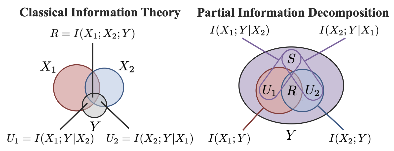
Partial Information Decomposition (PID) is an information-theoretic tool that formalizes this story by decomposing the total mutual information (I(X_1, X_2; Y)) into four nonnegative parts:

• Redundancy (R)
• Unique information in (X_1): (U_1)
• Unique information in (X_2): (U_2)
• Synergy (S)

with [ I(X_1, X_2; Y) = R + U_1 + U_2 + S. ]

---

The bottleneck: PID is expensive on modern data

A widely used definition of PID (e.g., the Bertschinger et al. formulation) expresses PID terms via optimization over a set of joint distributions that preserve two pairwise marginals ((X_1, Y)) and ((X_2, Y)).
That optimization becomes hard in the regimes we care about most: continuous, high-dimensional, non-Gaussian modalities.

So the practical goal is:

Keep the clean information-theoretic semantics of PID, but make it computable on real multimodal datasets.

---

Thin-PID: fast and exact Gaussian PID

Our first contribution is a theoretical result that unlocks an efficient solver:

Gaussian optimality: if the pairwise marginals are Gaussian, the GPID optimization admits an optimal jointly Gaussian solution.
Restricting the optimizer to joint Gaussians is not a relaxation—it is optimal.

Intuitively, this is powered by a classic entropy fact: among distributions with fixed second moments, Gaussians maximize differential entropy, which leads to tight conditional-entropy bounds under the constraints.

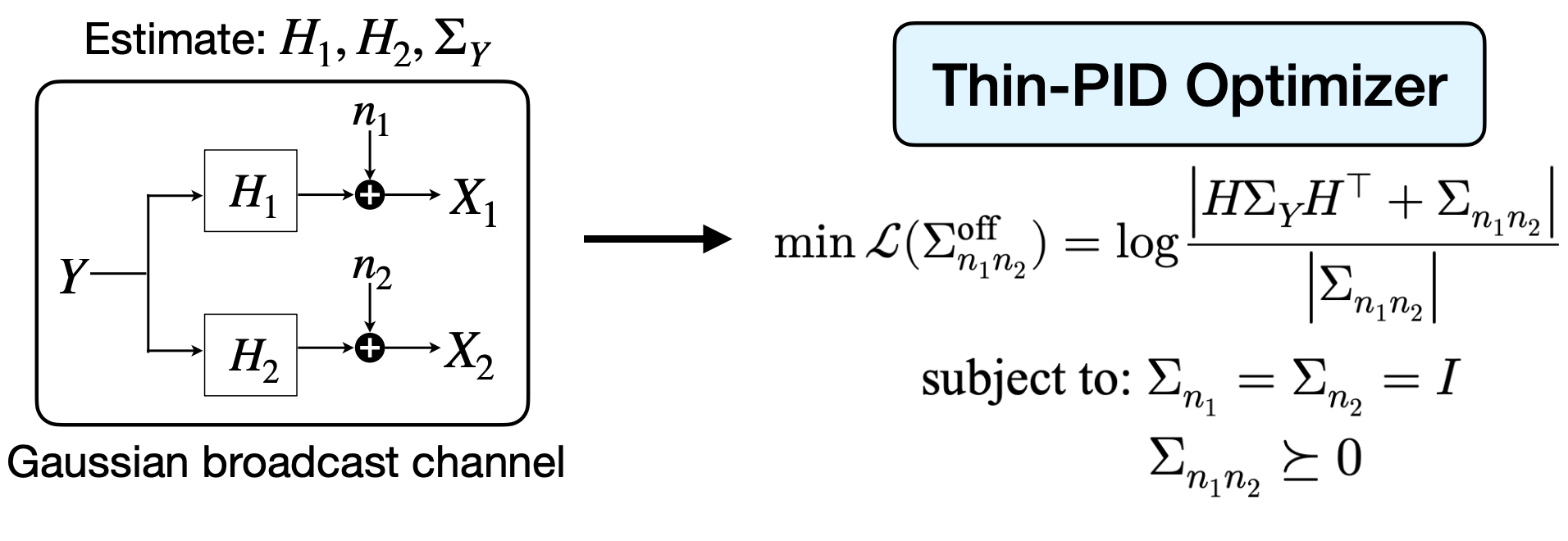
A broadcast-channel view: We reparameterize the Gaussian setting as a broadcast channel. [ X_1 = H_1 Y + n_1, \qquad X_2 = H_2 Y + n_2. ] After whitening, the remaining freedom lives largely in the cross-covariance between noises. The synergy computation becomes a clean log-determinant optimization with a PSD constraint, which we solve via projected gradient descent with stable SVD-based projections.

---

Flow-PID: extend GPID to non-Gaussian reality

Real-world modalities are rarely Gaussian. Flow-PID bridges this gap by learning invertible (bijective) transformations that map each variable into a latent space where the pairwise distributions are closer to Gaussian:

[ \hat X_1 = f_1(X_1),\quad \hat X_2 = f_2(X_2),\quad \hat Y = f_Y(Y), ] with (f_1, f_2, f_Y) implemented by normalizing flows.

Two facts make this a principled move:

• Mutual information is invariant under bijections (under mild regularity conditions).
• Under the same conditions, the PID structure is preserved in the transformed space.

So the pipeline is:

learn flows → obtain approximately Gaussian pairwise marginals in latent space → run Thin-PID to compute PID.

---

Limitations and future directions

Flow-PID depends on how well the learned bijections approximate Gaussian pairwise marginals; poor flow training (limited data, high complexity) can introduce estimation bias. Also, PID provides structural explanations of information interactions, not causal guarantees.

Looking ahead, I’m excited about using Flow-PID to guide dataset design (e.g., intentionally increasing synergy), to inform fusion-architecture choices, and potentially as a training signal/regularizer for multimodal representation learning.